Interpreting Real-Time PCR Amplification Plot

Quantitative real-time PCR (qPCR) has become a new normal in molecular biology for evaluating the gene expression. This technique allows for sensitive and specific detection of mRNA levels, forming the basis of transcriptomic studies. However, because RNA is dynamic and transient, especially when compared to the more stable DNA, optimizing the data analysis process is absolutely essential to obtain reproducible and meaningful results.

Unlike DNA, RNA’s presence and abundance fluctuate due to various biological conditions—making interpretation more nuanced. The true value of qPCR lies not just in the detection of gene expression, but in its precision, reproducibility, and context-aware interpretation.

Standard curves

To determine the copy number of a target sequence in absolute quantification qPCR, an accurately prepared standard curve is essential. This process begins with precise quantification of a known template before generating the curve. For example, if a template contains exactly 2 × 10¹¹ copies, it is serially diluted tenfold over eight steps, down to 2 × 10³ copies. Each dilution is then run in real-time PCR, typically with at least three replicates. The resulting Ct values are plotted to generate a standard curve, correlating specific Ct values to known copy numbers. The copy number in unknown samples is then calculated by comparing their Ct values to this curve.
The accuracy of absolute quantification in qPCR relies heavily on the consistency and reliability of the standard curve. Key considerations include:

• Template Quality and Quantification: The template used to generate the standard curve must be accurately quantified and highly pure, as it serves as the foundation for the entire experiment.
• Pipetting Precision: Accurate pipetting during the dilution series is critical, as even minor errors can lead to significant variability due to the high sensitivity of real-time PCR.
• Efficiency Matching: The reverse transcription and PCR amplification efficiencies must be consistent between the standard and experimental samples to ensure valid comparisons.

How to Generate a Standard Curve in qPCR:

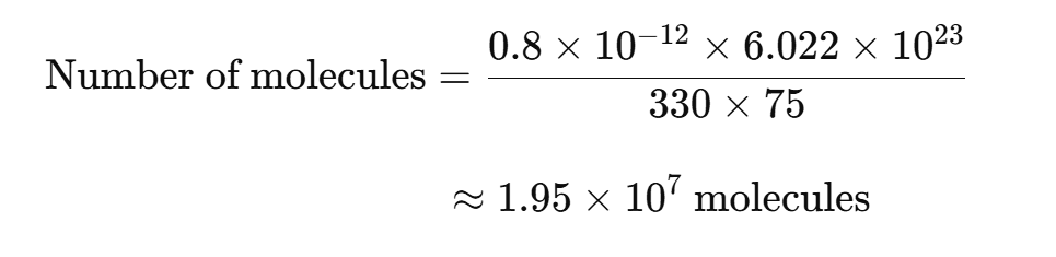
Start by determining the OD260 of the template sample. The template amount should be converted into molecule count using this formula:

For example, if a synthetic 75-mer oligonucleotide (single-stranded DNA) is used as the template, 0.8 pg would be equal to 2 × 10⁷ molecules:

How to Fix Missing or Strange Amplification Curves in qPCR Analysis

If no amplification curves or abnormal curves appear in your qPCR results, the first step is to verify the correct dye layer or reporter assignment. This is a common issue, especially on multi-user instruments and when templates are reused frequently.

For instance, using FAM and SYBR Green reporters with the same well recognition can cause overlapping spectra, making Ct values indistinguishable. To confirm the correct dye assignment, check the well’s Raw Spectra view with the “best match” option enabled. If the raw spectra don’t align with the expected curve, the wrong reporter is likely selected or there may be dye contamination.

To fix this, reassign the appropriate dye layer, update the wells, and reanalyze the data. Additionally, rebooting the data collection instrument between runs can help reset template parameters and reduce incorrect dye layer errors.

Understanding Contextual Variability in RNA Expression

RNA levels can differ dramatically across various cell types, developmental stages, and physiological or pathological states. This variability emphasizes the importance of controlling for biological and technical variables when analyzing mRNA expression.

To accurately interpret the transcriptome, it’s essential to account for:

• Tissue and cell specificity
• Developmental timing
• Physiological or pathological influences
• Environmental or experimental conditions

Only by considering these factors can the resulting data offer genuine biological insight.

Ensuring Technical Accuracy Before Biological Interpretation

Before diving into the biological implications of gene expression, it is critical to verify that technical aspects of the experiment are optimized:

• Check assay robustness — The qPCR assay should fulfill the key criteria for sensitivity, specificity, and reproducibility.
• Monitor contamination — Include no-template and negative controls.
• Account for genomic DNA contamination — Use exon-spanning primers or DNase treatment when necessary.

Key Components of a Robust qPCR Assay

A reliable assay will typically yield:

• Standard curve slope around -3.3 (reflecting ~100% efficiency)
• R² values ≥ 0.99 to confirm consistency
• Exponential amplification curves that cross the threshold within expected cycle ranges

To ensure this:

• Set the baseline and threshold correctly.
• Verify that amplification is within the detection range of your qPCR instrument.
• Validate with technical replicates to ensure data repeatability.

Amplification Curves and Their Interpretation

Amplification curves provides the visual proof of  qPCR’s outcomes:

• Normal curves show a flat baseline, sharp exponential rise, linear phase, and clear plateau.
• Abnormalities like jagged lines or “rainbow” arcs suggest errors in dye selection, contamination, or baseline miscalculation.

Troubleshooting Common Curve Issues:

Issue	Possible Cause	Fix
No curves	Wrong reporter dye	Reassign correct dye
Overlapping peaks	Cross-talk between dyes	Choose spectrally distinct dyes
Half-rainbows	Poor baseline settings	Adjust baseline 2–3 cycles below lowest Ct

The Role and Significance of Ct Values

The Ct (cycle threshold) is the PCR cycle number at which the fluorescence signal first rises above the background, indicating detectable levels of the target nucleic acid. It is influenced by:

• Baseline fluorescence
• Threshold placement
• Instrument software settings

Always ensure Ct values are due to genuine amplification. Remember that a genuine amplification can fail to generate a Ct if the baseline or threshold settings are incorrect.

Normalization Using Passive Reference Dyes

To account for well-to-well variability, the reporter signal is normalized using passive reference dyes like ROX. This leads to:

• Rn (Normalized Reporter Signal) = Reporter / Passive reference
• ΔRn (Corrected Normalized Signal) = Rn – Background

This normalization is essential for reliable quantitative comparisons.

Constructing and Validating Standard Curves

Standard curves  is the most crucial part of absolute quantification in qPCR. A well-constructed curve allows you to estimate unknown sample concentrations based on known template dilutions.

Steps to generate a standard curve:

1. Quantify your starting template precisely (e.g., using OD260 for nucleic acids).
2. Convert mass to molecule number using molecular weight.
3. Perform serial 10-fold dilutions (e.g., from 2×10¹¹ to 2×10³ copies).
4. Run each dilution in triplicate.
5. Plot Ct vs log(copy number) to create the standard curve.

Ensure that:

• Pipetting is accurate throughout.
• In qPCR, using a template for the standard curve that closely matches the experimental target ensures accurate and consistent quantification.
• The slope (~−3.3), R², and y-intercept confirm high assay efficiency and reproducibility.

Best Practices for Absolute Quantification

Absolute quantification measures exact copy numbers, but its accuracy hinges on:

• Accurate quantification of standard templates.
• Consistent reverse transcription and PCR efficiency across all samples and standards ensures reliable qPCR results.
• Minimized human error, especially during serial dilutions.

Even tiny inconsistencies in pipetting or mixing can lead to significant deviations due to the sensitivity of qPCR.

Baseline Settings and Adjustment Strategies

The baseline represents the background fluorescence signals in the PCR reaction before exponential amplification begins. Incorrect baseline settings can distort the data, leading to:

• False positive Ct values
• Flat or noisy curves
• “Rainbow” patterns, visible arcs on the curve between cycles 1–10

Best practices:

• Set the upper baseline limit 2–3 cycles below the lowest Ct.
• Use linear scale plots to better visualize curve alignment.
• Adjust as needed to ensure consistent curve shapes across replicates.

When baseline anomalies persist, examine the Raw Spectra or Multicomponent views to determine if there’s genuine amplification or just noise.

Threshold Settings for Reliable Analysis

The threshold is a fixed fluorescence level that the reaction must cross to be considered positive. It is usually set during exponential phase of amplification.

Key points:

• Don’t adjust the threshold until the baseline is properly set.
• Most platforms use 10 standard deviations above baseline as default.
• In low abundance targets, multiple thresholds may be needed.

Some labs use methods like the Second Derivative Maximum (SDM) to determine the point of greatest slope, improving consistency.

Comparative Quantification Using ΔΔCt Method

This widely used method evaluates gene expression changes by comparing:

• Test sample vs calibrator (e.g., untreated control)
• Target gene vs reference gene (e.g., GAPDH, ACTB)

Formula:

ΔCt = Ct(GOI) – Ct(Norm)
ΔΔCt = ΔCt(Test) – ΔCt(Calibrator)
Fold Change = 2^-ΔΔCt

Ensure that:

• Target and reference genes have almost similar PCR efficiencies.
• Efficiencies are validated by plotting ΔCt vs log(dilution factor) — a flat line indicates matched efficiencies.

Advanced Approach: Standard Curve-Based Comparative Quantification

This method refines ΔΔCt analysis by incorporating efficiency correction:

• Build standard curves for both target and reference genes.
• Normalize Ct values to reference gene and correct for minor efficiency differences.

This approach is more precise and avoids assumptions made in the traditional ΔΔCt method. It is particularly useful when exact quantification is required or when comparing across different runs or instruments.

High Resolution Melting (HRM) Curve Analysis

HRM is a powerful, post-PCR method used to detect:

• SNPs (Single Nucleotide Polymorphisms)
• Small mutations
• DNA methylation patterns

Process:

1. Amplify 80–250 bp fragments with a high-performance dsDNA-binding dye.
2. Heat the product slowly while monitoring fluorescence.
3. Measure melting temperature (Tm) which then generates melting curves.

Benefits of HRM:

• Closed-tube, contamination-free detection
• High sensitivity to even single base changes
• Ideal for mutation scanning and genotyping

Multiplex Real-Time PCR Techniques

Multiplexing allows simultaneous amplification of multiple targets in one reaction, saving time and reagents.

Advantages:

• Reduces well-to-well variability
• Minimizes reagent usage and cost
• Enhances experimental throughput

Challenges:

• Designing compatible primers and probes
• Avoiding target interference
• Balancing amplification efficiencies

Use spectrally distinct dyes and validate that each target amplifies efficiently without competing with others.

Managing Fluorophore/Quencher Combinations in Multiplexing

In multiplex qPCR, fluorophores and quenchers must be carefully selected to avoid signal overlap:

• Choose spectrally distinct fluorophores (e.g., FAM, HEX, Cy5)
• Avoid cross-talk between dyes by ensuring emission filters are compatible with the dyes used.
• Use dark quenchers like NFQ or QSY to minimize background noise.
• Avoid TAMRA in multiplexing, as it emits fluorescence and complicates signal detection. Dark quenchers dissipate energy as heat, improving accuracy.

Frequently Asked Questions (FAQs)

1. What causes inconsistent amplification curves in qPCR?
   Poor dye selection, baseline errors, or template contamination can lead to jagged or flat curves. Always confirm reporter assignment and adjust the baseline.
2. How can I validate qPCR efficiency?
   Use a standard curve and calculate slope; a value of −3.3 indicates 100% efficiency. R² should be ≥ 0.99.
3. Why is baseline setting so critical in qPCR?
   Incorrect baselines can cause false Ct values, misrepresenting true expression. Set the baseline 2–3 cycles below the lowest Ct.
4. Can I use different thresholds for different targets in multiplex qPCR?
   Yes, especially when targets have vastly different expression levels. Use separate thresholds as needed but interpret results cautiously.
5. What is the best way to normalize qPCR data?
   Use internal reference genes (e.g., RNAseP, GAPDH) and normalize using ΔCt or ΔΔCt methods. Verify that reference gene expression is stable across all samples.
6. Is high-resolution melting (HRM) better than conventional melt curves?
   Yes. HRM provides higher sensitivity and precision for mutation detection and requires no post-PCR handling.

Conclusion

qPCR is a robust and powerful technique, but only when data analysis is done meticulously. From baseline and threshold settings to curve interpretation and normalization strategies, every step plays a vital role in ensuring accurate and biologically meaningful results.

By following the best practices outlined here—constructing high-quality standard curves, validating efficiencies, normalizing correctly, and avoiding common pitfalls—you can optimize qPCR data analysis and significantly enhance the reliability of your gene expression studies.